Exponential curve fitting using R

[Glug]

Hiya Folks,

Estimating tuning or mussette tuning has come up a few times and I've occasionally piped up and mentioned a (free) stats package that will do it.
So here's some info (updated to the latest release).

Stats package: R https://www.r-project.org/
latest verion is 4.3.2

Additional libraries: ggplot2, ggtrendline
ggtrendline is the current replacement for basicTrendline

Installation:
R itself is fairly easy - just download the install file from the web site.
You then need to add a couple of packages:
1) Start R (as administrator on Windows)
2) Packages / Install package(s) from the menu
3) Select a repository
4) Select 'ggplot2' or 'ggtrendline'
NB. you need to add both ggplot2 and ggtrendline

Example:
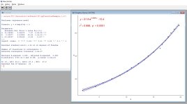
To run the example you do File / Source R code and select the example file (ggTrendlineexample.1.r)
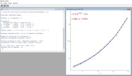
You should then get



That example is actually a bicycle spoke tension meter (because it's very exponential) but all you need to do is edit the file and put your own data in there.

This package will actually do several models:
"line2P" (formula as: y=a*x+b),
"line3P" (y=a*x^2+b*x+c),
"log2P" (y=a*ln(x)+b),
"exp2P" (y=a*exp(b*x)),
"exp3P" (y=a*exp(b*x)+c),
"power2P" (y=a*x^b),
"power3P" (y=a*x^b+c).

I've attached the example in a zip file, but it's just a text (*.r) file that looks like this:
#
# See https://github.com/PhDMeiwp/ggtrendline
#
library(ggplot2)
library(ggtrendline)

# Lucia IV P
#
# line2P: y = 1.56171 + 0.14853 x Rsq = 0.967
# exp3P: y = 27.08940 - 25.65090 exp (-0.00655 x) Rsq = 0.968
#
# x <- 1:37
# y <- c(1.7, 1.7, 1.85, 2.1, 2.15, 2.4, 2.55, 2.7, 3.1, 3.05, 3.1, 3.6, 3.4, 3.65, 3.95, 4.25, 4.25, 4.55, 4.5, 4.65, 4.35, 4.55, 5.2, 5.35, 5.25, 5.35, 5.15, 6.15, 5.5, 6.35, 5.85, 6.2, 6.9, 6.4, 6.45, 6.1, 7.9)


# Ztto TC-1
#
# exp3P: kgf = -10.42037 + 21.86882 * exp (0.08278 * reading)
#
x <- c(1.9, 4.3, 5.7, 7.3, 8.8, 10.2, 10.9, 12.2, 13.3, 14, 15, 16.2, 16.6, 17.2, 17.7, 18.2, 18.8, 19.7)
y <- c(15, 20, 25, 30, 35, 40, 45, 50, 55, 60, 65, 70, 75, 80, 85, 90, 95, 100)


# print (ggtrendline(x, y, model="line2P", linecolor="blue", linetype=1, linewidth=1, eSize=5, text.col="red") + geom_point(aes(x, y)) + theme_classic())
print (ggtrendline(x, y, model="exp3P", linecolor="blue", linetype=1, linewidth=1, eSize=5, text.col="red") + geom_point(aes(x, y)) + theme_classic())

 

[Jeremyh]

I'm a Python user myself, I imagine you could do the same using the matplotlib and either pandas or numpy/scipy libraries.

 

[JeffJetton]

Very cool!

FWIW, if you didn't want to install any packages (not that that's hard to do or anything), you could pull off something similar just using base R. This is equivalent to "exp2P", for example:

x <- c(1.9, 4.3, 5.7, 7.3, 8.8, 10.2, 10.9, 12.2, 13.3, 14, 15, 16.2, 16.6, 17.2, 17.7, 18.2, 18.8, 19.7)
y <- c(15, 20, 25, 30, 35, 40, 45, 50, 55, 60, 65, 70, 75, 80, 85, 90, 95, 100)

# Take log of y to turn a linear model into exponential model
fit <- lm(log(y) ~ x)
summary(fit)

# Take exponent of predictions to transform everything back
preds <- exp(predict(fit, data=data.frame(x, y), interval="confidence"))

# Show original data points
plot(x, y, pch=19)
# Overlay trendline (first column of preds) and confidence intervals (cols 2 & 3)
matplot(x, preds, type="l", add=TRUE,
        col=c("blue", "red", "red"),
        lty=c(1, 3, 3))

Granted, the point of the package is that it handles so much of that for you automatically, which is very nice!

 

[JeffJetton]

I'm a Python user myself, I imagine you could do the same using the matplotlib and either pandas or numpy/scipy libraries.

Yup. And in fact I wonder if someone has done a similar Python package with all the bells and whistles of ggtrendline?

For those who aren't keen to fool with either R or Python, you could do a basic exponential model using Excel, using the same idea in my R example above:

1. Put your x and y values in cells
2. Add a column that takes the log of your y values
3. Use the SLOPE() and INTERCEPT() formulas to get the coefficients of a linear model log given x.
4. Add a column of exp(slope*x + intercept) to get predicted y values
5. Chart away!

Even easier, you can insert a scatterplot of your x and y values, then add an exponential trendline to the chart (may require a bit of digging around the menus to find the option). Excel will give you an option to show the resulting formula as well as the R-squared. (No confidence interval though.)

 

[pitzelberger]

I have done an ipython notebook some time ago